geoDB Access
The geoDB is a service provided by the Euro Data Cube project (EDC) as a payed service. It comes with a Python client that provides hugh level acess to your data and a certain amount of space in a PostGreSQL database. For exploring data you will need at least a read only to the geoDB which you can purchase at the EDC market place.
You can access the service in two ways:
By using the Jupyter Python notebook provided by EDC Marketplace (configuartion free,
geodb = GeoDBClient())By using you own Jupyter notebook or Python script by providing a client id and secret to the GeoDBClient (
geodb = GeoDBClient(client_id="myid", client_secret="mysecet"))
The client ID and secret is also provided by EDC in the latter case. You will find them in your EDC Marketplace account section. You can also provide the credentials via system environment varibles (GEODB_AUTH_CLIENT_ID and GEODB_AUTH_CLIENT_SECRET). These variables can be supplied via a .env file.
Exploring Data
[1]:
from xcube_geodb.core.geodb import GeoDBClient
Login from any maschine
Install xcube geoDB with command:
conda install xcube_geodb -c conda-forge
[20]:
### uncomment if not on EDC
#client_id=YourID
#client_secret=YourSecret
#geodb = GeoDBClient(client_id=client_id, client_secret=client_secret, auth_mode="client-credentials")
Login in EDC environment
[21]:
### comment if not on EDC

geodb = GeoDBClient()
Get your user name
[3]:
geodb.whoami
[3]:
'geodb_ci_test_user'
[4]:
geodb.get_my_collections()
[4]:
| owner | database | table_name | |
|---|---|---|---|
| 0 | geodb_9bfgsdfg-453f-445b-a459 | geodb_9bfgsdfg-453f-445b-a459 | land_use |
| 1 | tt | tt | tt300 |
[5]:
import geopandas

# Have a look at fiona feature schema
collections = {
        "land_use":
        {
            "crs": 3794,
            "properties":
            {
                "RABA_PID": "float",
                "RABA_ID": "float",
                "D_OD": "date"
            }
        }
    }


geodb.create_collections(collections, clear=True)
[5]:
{'collections': {'geodb_ci_test_user_land_use': {'crs': 3794,
                                                 'properties': {'D_OD': 'date',
                                                                'RABA_ID': 'float',
                                                                'RABA_PID': 'float'}}}}
[6]:
gdf = geopandas.read_file('data/sample/land_use.shp')
geodb.insert_into_collection('land_use', gdf.iloc[:100,:]) # minimizing rows to 100, if you are in EDC, you dont need to make the subset.
Processing rows from 0 to 100
[6]:
100 rows inserted into land_use
List Datasets
Step 1: List all datasets a user has access to.
[7]:
geodb.get_my_usage() # to be updated so that all available collections are displayed includign sensible information ont heir availability, e.g. public, purchased, etc..
[7]:
{'usage': '96 kB'}
[8]:
geodb.get_my_collections()
[8]:
| owner | database | table_name | |
|---|---|---|---|
| 0 | geodb_9bfgsdfg-453f-445b-a459 | geodb_9bfgsdfg-453f-445b-a459 | land_use |
| 1 | geodb_ci_test_user | geodb_ci_test_user | land_use |
| 2 | tt | tt | tt300 |
Step 2: Let’s get the whole content of a particular data set.
[9]:
gdf = geodb.get_collection('land_use') # to be updated, so that namespace is not needed or something more suitable, e.g. 'public'
gdf
[9]:
| id | created_at | modified_at | geometry | raba_pid | raba_id | d_od | |
|---|---|---|---|---|---|---|---|
| 0 | 1 | 2021-01-22T10:02:34.390867+00:00 | None | POLYGON ((453952.629 91124.177, 453952.696 911... | 4770326 | 1410 | 2019-03-26 |
| 1 | 2 | 2021-01-22T10:02:34.390867+00:00 | None | POLYGON ((453810.376 91150.199, 453812.552 911... | 4770325 | 1300 | 2019-03-26 |
| 2 | 3 | 2021-01-22T10:02:34.390867+00:00 | None | POLYGON ((456099.635 97696.070, 456112.810 976... | 2305689 | 7000 | 2019-02-25 |
| 3 | 4 | 2021-01-22T10:02:34.390867+00:00 | None | POLYGON ((455929.405 97963.785, 455933.284 979... | 2305596 | 1100 | 2019-02-25 |
| 4 | 5 | 2021-01-22T10:02:34.390867+00:00 | None | POLYGON ((461561.512 96119.256, 461632.114 960... | 2310160 | 1100 | 2019-03-11 |
| ... | ... | ... | ... | ... | ... | ... | ... |
| 95 | 96 | 2021-01-22T10:02:34.390867+00:00 | None | POLYGON ((458514.067 93026.352, 458513.306 930... | 5960564 | 1600 | 2019-01-11 |
| 96 | 97 | 2021-01-22T10:02:34.390867+00:00 | None | POLYGON ((458259.239 93110.981, 458259.022 931... | 5960569 | 3000 | 2019-01-11 |
| 97 | 98 | 2021-01-22T10:02:34.390867+00:00 | None | POLYGON ((458199.608 93099.296, 458199.825 930... | 5960630 | 3000 | 2019-01-11 |
| 98 | 99 | 2021-01-22T10:02:34.390867+00:00 | None | POLYGON ((458189.403 93071.618, 458179.669 930... | 5960648 | 1100 | 2019-01-11 |
| 99 | 100 | 2021-01-22T10:02:34.390867+00:00 | None | POLYGON ((454901.777 95801.099, 454889.964 958... | 2353305 | 1321 | 2019-01-05 |
100 rows × 7 columns
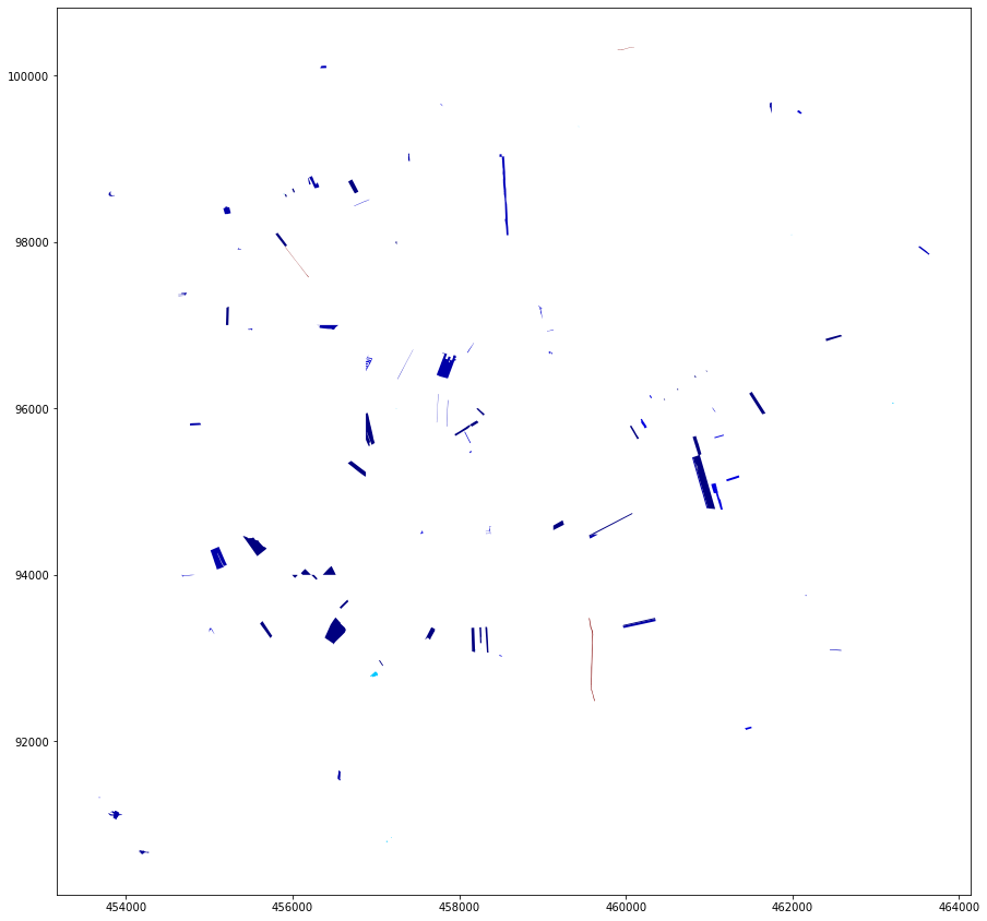
Step 3: Plot the GeoDataframe, select a reasonable column to diplay
[10]:
gdf.plot(column="raba_id", figsize=(15,15), cmap = 'jet')
[10]:
<matplotlib.axes._subplots.AxesSubplot at 0x7f323b4fa190>
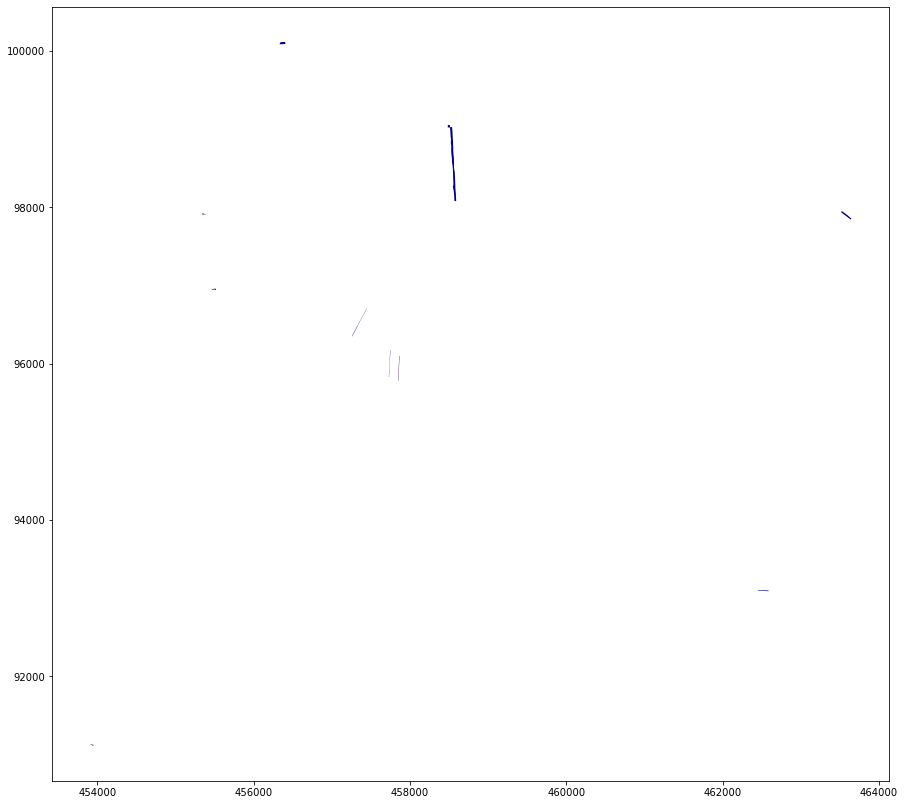
Step 5: Subselect the data. Here: Select a specific use by defining an ID value to choose
[11]:
gdfsub = geodb.get_collection('land_use', query='raba_id=eq.1410')
gdfsub.head()
[11]:
| id | created_at | modified_at | geometry | raba_pid | raba_id | d_od | |
|---|---|---|---|---|---|---|---|
| 0 | 1 | 2021-01-22T10:02:34.390867+00:00 | None | POLYGON ((453952.629 91124.177, 453952.696 911... | 4770326 | 1410 | 2019-03-26 |
| 1 | 62 | 2021-01-22T10:02:34.390867+00:00 | None | POLYGON ((457261.001 96349.254, 457256.831 963... | 3596498 | 1410 | 2019-01-05 |
| 2 | 22 | 2021-01-22T10:02:34.390867+00:00 | None | POLYGON ((455384.809 97907.054, 455380.659 979... | 3616776 | 1410 | 2019-02-25 |
| 3 | 28 | 2021-01-22T10:02:34.390867+00:00 | None | POLYGON ((462585.734 93088.987, 462567.020 930... | 3826126 | 1410 | 2019-01-23 |
| 4 | 32 | 2021-01-22T10:02:34.390867+00:00 | None | POLYGON ((457748.827 96167.354, 457748.394 961... | 2309744 | 1410 | 2019-01-05 |
[12]:
gdfsub.plot(column="raba_id", figsize=(15,15), cmap = 'jet')
[12]:
<matplotlib.axes._subplots.AxesSubplot at 0x7f323b199190>
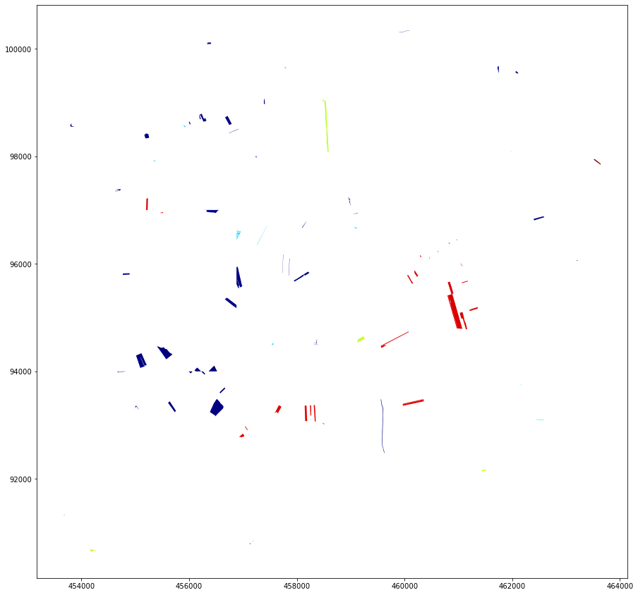
Step 6: Filter by bbox, limit it to 200 entries
[13]:
gdf = geodb.get_collection_by_bbox(collection="land_use",  bbox = (452750.0, 88909.549, 464000.0, 102486.299), comparison_mode="contains", bbox_crs=3794, limit=200, offset=10)
gdf
[13]:
| id | created_at | modified_at | geometry | raba_pid | raba_id | d_od | |
|---|---|---|---|---|---|---|---|
| 0 | 11 | 2021-01-22T10:02:34.390867+00:00 | None | POLYGON ((460137.998 95628.898, 460111.001 956... | 5983161 | 1100 | 2019-03-11 |
| 1 | 12 | 2021-01-22T10:02:34.390867+00:00 | None | POLYGON ((453673.609 91328.224, 453678.929 913... | 5983074 | 1600 | 2019-03-26 |
| 2 | 13 | 2021-01-22T10:02:34.390867+00:00 | None | POLYGON ((460312.295 96127.114, 460300.319 961... | 5983199 | 1600 | 2019-03-11 |
| 3 | 14 | 2021-01-22T10:02:34.390867+00:00 | None | POLYGON ((460459.445 96117.356, 460470.516 961... | 5983217 | 1100 | 2019-03-11 |
| 4 | 15 | 2021-01-22T10:02:34.390867+00:00 | None | POLYGON ((457798.753 99628.982, 457783.076 996... | 6299143 | 1600 | 2019-03-04 |
| ... | ... | ... | ... | ... | ... | ... | ... |
| 85 | 96 | 2021-01-22T10:02:34.390867+00:00 | None | POLYGON ((458514.067 93026.352, 458513.306 930... | 5960564 | 1600 | 2019-01-11 |
| 86 | 97 | 2021-01-22T10:02:34.390867+00:00 | None | POLYGON ((458259.239 93110.981, 458259.022 931... | 5960569 | 3000 | 2019-01-11 |
| 87 | 98 | 2021-01-22T10:02:34.390867+00:00 | None | POLYGON ((458199.608 93099.296, 458199.825 930... | 5960630 | 3000 | 2019-01-11 |
| 88 | 99 | 2021-01-22T10:02:34.390867+00:00 | None | POLYGON ((458189.403 93071.618, 458179.669 930... | 5960648 | 1100 | 2019-01-11 |
| 89 | 100 | 2021-01-22T10:02:34.390867+00:00 | None | POLYGON ((454901.777 95801.099, 454889.964 958... | 2353305 | 1321 | 2019-01-05 |
90 rows × 7 columns
[14]:
gdf.plot(column="raba_pid", figsize=(15,15), cmap = 'jet')
[14]:
<matplotlib.axes._subplots.AxesSubplot at 0x7f323b11b090>
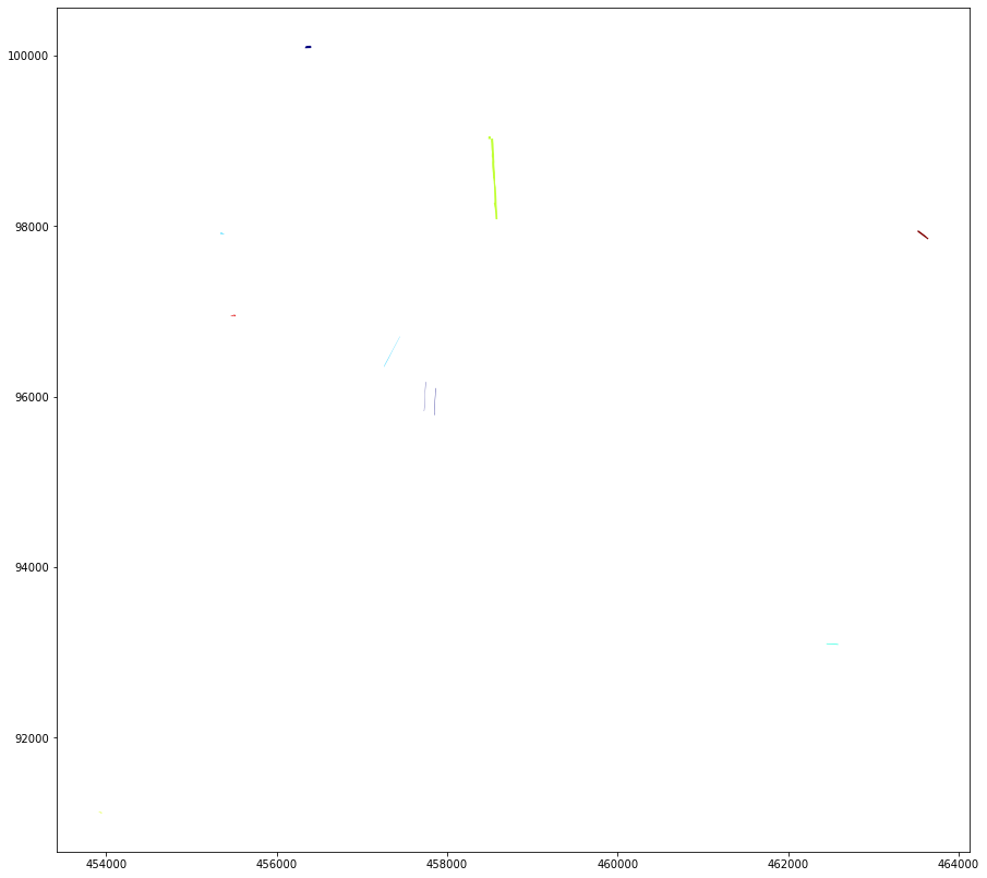
Step 6: Fltering using PostGres Syntax; see https://www.postgresql.org/docs/9.1/index.html for details
[15]:
gdf = geodb.get_collection_pg(collection='land_use', where='raba_id=1410')
gdf.head()
[15]:
| id | created_at | modified_at | geometry | raba_pid | raba_id | d_od | |
|---|---|---|---|---|---|---|---|
| 0 | 1 | 2021-01-22T10:02:34.390867+00:00 | None | POLYGON ((453952.629 91124.177, 453952.696 911... | 4770326 | 1410 | 2019-03-26 |
| 1 | 62 | 2021-01-22T10:02:34.390867+00:00 | None | POLYGON ((457261.001 96349.254, 457256.831 963... | 3596498 | 1410 | 2019-01-05 |
| 2 | 22 | 2021-01-22T10:02:34.390867+00:00 | None | POLYGON ((455384.809 97907.054, 455380.659 979... | 3616776 | 1410 | 2019-02-25 |
| 3 | 28 | 2021-01-22T10:02:34.390867+00:00 | None | POLYGON ((462585.734 93088.987, 462567.020 930... | 3826126 | 1410 | 2019-01-23 |
| 4 | 32 | 2021-01-22T10:02:34.390867+00:00 | None | POLYGON ((457748.827 96167.354, 457748.394 961... | 2309744 | 1410 | 2019-01-05 |
[16]:
gdf.plot(column="raba_pid", figsize=(15,15), cmap = 'jet')
[16]:
<matplotlib.axes._subplots.AxesSubplot at 0x7f323b13a9d0>
Step 7: Fltering using PostGres Syntax Allowing Aggregation Here according to data, note that the data set has been reduced to 200 entries above
[17]:
df = geodb.get_collection_pg('land_use', where='raba_id=1410', group='d_od', select='COUNT(d_od) as ct, d_od')
df.head()
[17]:
| ct | d_od | |
|---|---|---|
| 0 | 1 | 2019-03-04 |
| 1 | 1 | 2019-03-20 |
| 2 | 1 | 2019-03-26 |
| 3 | 1 | 2019-04-01 |
| 4 | 1 | 2019-02-25 |
[18]:
geodb.drop_collection('land_use')
[18]:
Collection ['geodb_ci_test_user_land_use'] deleted
[ ]:
[ ]: